Process Identification & PID Tuning Tool

Problem

PID loops on plant get tuned by feel. An engineer bumps the output, watches the trend, adjusts a gain, and moves on. The result is undocumented, unrepeatable, and impossible to compare between loops or between commissioning visits.

Meanwhile the data needed to do it properly is already being historised — the step tests are recorded, nobody analyses them.

My role & scope

Sole designer and developer: the numerical core, the historian queries and the web interface. Used for analysis of cascade control loops.

Approach

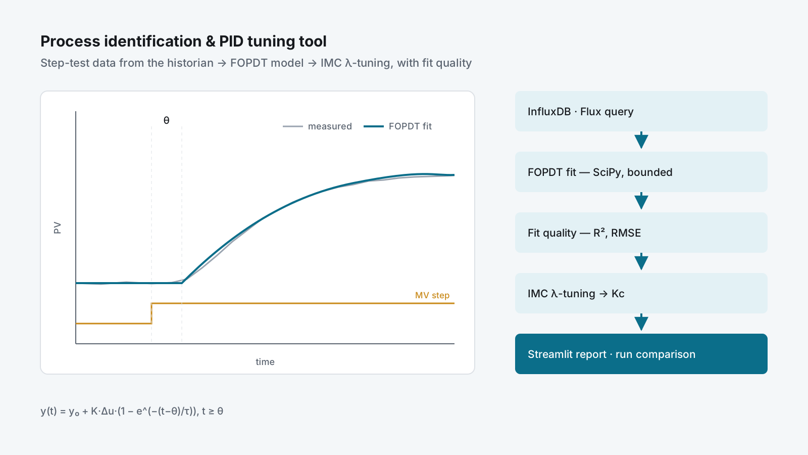
A web tool that reads step-test data straight out of the process historian, fits a first-order plus dead-time model to it, reports how good the fit actually is, and produces tuning parameters from that model.

InfluxDB (Flux query)  →  step-response series
        ↓
FOPDT model fit (SciPy curve_fit, bounded, seeded)
        ↓
Fit quality (R², RMSE)  +  performance metrics
        ↓
IMC λ-tuning  →  controller gain
        ↓
Multi-run comparison table + overlaid Plotly trends

Model identification

The process is fitted to a first-order plus dead-time model:

y(t) = y₀ + K·Δu·(1 − e^(−(t−θ)/τ))    for t ≥ θ

Rather than throwing the raw data at an optimiser and hoping, the fit is seeded from a classical graphical estimate — the 28.3 % and 63.2 % response crossings give a starting τ and θ — and then refined by bounded non-linear least squares. Bounds keep the gain sign consistent with the move direction and keep dead time physically plausible. If the optimiser fails to converge, the tool falls back to the graphical estimate rather than returning nothing.

Reported metrics

Group	Values
Model	K (process gain), τ (time constant), θ (dead time)
Fit quality	R², RMSE — is this model worth trusting?
Tuning	λ (IMC filter time), Kc (controller gain)
Response	rise time (10→90 %), settling time (±2 %), overshoot %, error at 3τ
Test conditions	MV before/after, ΔMV, PV before/after

A tuning number without an R² beside it is an opinion; with one, it is a measurement.

Comparison workflow

Multiple runs are loaded as named tests, each with its own measurement, field and time window, then compared side by side in one table with trends overlaid. That answers “did this loop degrade since last year?” and “which of these tuning candidates is actually better?” with evidence. The λ factor is adjustable, so the speed-versus-robustness trade-off is a visible choice.

Delivery

Working tool, used for analysis of cascade control loops. Planned hardening:

• Configuration via environment variables rather than in-code defaults
• Type hints and a pytest suite over the numerical core
• Core library separated from the Streamlit UI so it can be called from a pipeline
• Containerised deployment alongside the historian

Result

• Loop tuning backed by a fitted model and a fit-quality figure, not by feel
• A record of each step test that survives the site visit
• Side-by-side comparison of runs to see loop degradation over time

Skills used

Process control theory (FOPDT identification, IMC λ-tuning, cascade loops) · Python — SciPy, pandas, Plotly, Streamlit · InfluxDB / Flux · turning control theory into a tool commissioning engineers can use on site.